Q: 1 What is/are the uses of “Macro Feature” in MS-Excel?
1. It is used to send messages.
2. It saves a lot of time.
3. It designs the work sheet.
4. It maintains the uniformity of formatting changes in a sheet.
Choose the most appropriate answer from the options given below:
3 only
2 only
1 and 4 only
2 and 4 only
[ Option D ]
Macro is a feature in MS Excel that records a sequence of actions so that they can be automatically (saves time) repeated later. It is mainly used to automate repetitive tasks and maintain consistency (uniformity) in formatting or calculations.
Q: 2 In MS Excel 2019, which of the following operator has the highest precedence?
+
^
&
%
[ Option D ]
The Percent (%) operator actually has a higher precedence than ^ (Exponentiation) and operates immediately after evaluating the number it follows.
Q: 3 Which of the following is NOT a function of MS Excel?
count()
min()
max()
subtract()
[ Option D ]
MS Excel supports many built-in functions for calculations and data analysis. Functions like count(), min(), and max() are all valid and are used to count items, find the minimum value, and find the maximum value in data, respectively.
| FUNCTION | PURPOSE | EXAMPLE | RESULT |
|---|---|---|---|
| SUM() | Adds numbers in a range. | =SUM(2, 4, 8) | 14 |
| AVERAGE() | Finds the average (mean) of numbers. | =AVERAGE(10, 20, 30) | 20 |
| COUNT() | Counts numeric values in a range. | =COUNT(54, "suraku", 74) | 2 |
| COUNTA() | Counts all non-empty cells including numbers and text. | =COUNTA(54, "suraku", 74) | 3 |
| MIN() | Finds the smallest value. | =MIN(10, 22, 18) | 10 |
| MAX() | Finds the largest value. | =MAX(10, 12, 8) | 12 |
| PRODUCT() | Multiplies numbers. | =PRODUCT(2, 3, 5) | 30 |
| SQRT() | Returns the square root. | =SQRT(25) | 5 |
| POWER() | Raises a number to a power. | =POWER(2, 3) | 8 |
| MOD() | Returns the remainder after division. | =MOD(10, 3) | 1 |
Q: 4 The default font for MS Excel 2019 datasheet is?
Arial 11 point
Arial Black 11 point
Calibri 11 point
Times New Roman 11 point
[ Option C ]
The Calibri with a font size of 11 points has been the default font in Microsoft Office (Word, Excel, PowerPoint) since Office 2007, replacing Times New Roman.
Q: 5 A valid formula is Excel begins with –
+
=
#
@
[ Option B ]
In Microsoft Excel, a formula is an expression used to perform calculations or other actions on data in worksheet cells. Every valid Excel formula begins with an Equal Sign (=), which signals to Excel that the cell contains a formula, not just plain text, or numbers.
Remember:
Q: 6 Which is not a commonly used type of cell data in Spreadsheet?
Numeric Value
Date and Time
User Authentication
Label and Formula
[ Option C ]
User Authentication is not a type of data input in spreadsheets. Authentication relates to verifying user identity and is handled by security systems, not by spreadsheet data entry.
| Data Type | Description |
|---|---|
| Numeric Value | Numbers used for calculations. |
| Text / Label | Words or text used for names, headings, or categories. |
| Date and Time | Stores calendar dates and times in proper format. |
| Formula | Equations that calculate values based on cell references. |
| Boolean / Logical | Represents logical values (TRUE or FALSE), used in conditions and logical formulas. |
Q: 7 What will be the output of the following in MS-Excel?
=LCM(5,7,35)
70
1225
12
35
[ Option D ]
In MS Excel, the LCM function is used to calculate the Least Common Multiple of one or more numbers. The LCM is the smallest number that is divisible by all the given numbers with remainder 0. For example, the formula =LCM(5, 7, 35) calculates the LCM of 5, 7, and 35.
Q: 8 In Excel 2016, if you want to insert 3 columns between Column G and H you would-
Select column G and right click and select insert for 3 times
Select column H and right click and select insert for three times
Select column E, F and G and right click and select insert for three times
Select column D, E and F and right click and select insert for three times
[ Option B ]
In Excel 2016, when you want to insert multiple columns, it is important to understand that Excel always inserts new columns to the left of the selected column(s).
To insert 3 columns between Column G and H, we need to select Column H first. By right-clicking and choosing Insert, a new column will appear to the left of H. Repeating this process three times will insert three new columns exactly between G and H.
Q: 9 Consider the Excel formula for the Excel Sheet –
| A | B | C | D | E | |
|---|---|---|---|---|---|
| 1 | 60 | A1 | 75 | A1 | =if(A1=C1,”T”,”F”) |
| 2 | 70 | A2 | 70 | A2 | =if(A2=C2,”T”,”F”) |
| 3 | 90 | A3 | 90 | A3 | =if(B3=D3,”T”,”F”) |
What will be the output in column no.5?
| F |
| F |
| F |
| T |
| T |
| F |
| F |
| T |
| T |
| T |
| T |
| T |
[ Option C ]
Q: 10 Which of the following in spreadsheet is a method of arranging the data in ascending or descending order?
Filter
Sorting
Auto Sum
Logical Operator
[ Option B ]
Sorting in a spreadsheet like MS Excel, refers to arranging data in a specific order, either ascending (smallest to largest or A to Z) or descending (largest to smallest or Z to A). This helps organize data logically for easier analysis and viewing.
Q: 11 “Pivot Table” is a feature of which of the following software?
Microsoft Excel
Microsoft Word
Microsoft Access
Microsoft Powerpoint
[ Option A ]
A Pivot Table is a powerful feature in Microsoft Excel used to summarize, analyze, explore, and present large sets of data quickly. Pivot Tables let users drag and drop fields to quickly change reports and analyze data trends interactively.
| Feature | Purpose |
|---|---|
| Pivot Table | Summarize and analyze large sets of data quickly. |
| VLOOKUP / HLOOKUP | Search and retrieve data vertically or horizontally. |
| Conditional Formatting | Highlight cells automatically based on rules or conditions. |
| Goal Seek (What-If Analysis) | Find input value required to achieve a desired result. |
| Macros | Automate repetitive tasks using VBA. |
| Data Validation | Restrict or control data entry in cells. |
| Filter / Advanced Filter | Display only rows that meet criteria. |
| Freeze Panes | Keep rows/columns visible while scrolling. |
| Text to Columns | Split one column’s data into multiple columns. |
| PMT Function | Calculate loan repayments / EMI. |
Q: 12 Microsoft Excel’s formula begins with ____________.
.
=
*
|
[ Option B ]
In Microsoft Excel, a formula is an expression used to perform calculations or other actions on data in worksheet cells. Every valid Excel formula begins with an Equal Sign (=), which signals to Excel that the cell contains a formula, not just plain text, or numbers.
Remember:
Q: 13 Which of the following is the most appropriate for the name of Excel Sheet?
Minimum 1 Character, Maximum 21 Character
Minimum 1 Character, Maximum 31 Character
Minimum 2 Character, Maximum 19 Character
Minimum 2 Character, Maximum 27 Character
[ Option B ]
In Microsoft Excel, a Workbook (Excel file) contains one or more Worksheets (commonly called "sheets"). Each sheet has a name, shown on the sheet tab at the bottom (like Sheet1, Sheet2, etc.). Users can rename sheets to give them meaningful names (like RSSB_Questions, RPSC_Questions, etc.).
When naming an Excel worksheet (sheet), the name must have at least 1 character (it cannot be left blank) and name cannot exceed 31 characters. The name cannot contain certain characters like:
Q: 14 Representation of data in a graphical manner is an important feature of Excel. Identify it. Also give the name of the component depicted below:
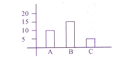
Image, Bar
Graph, Column
Graph, Bar
Graph, Column
[ Option D ]
Q: 15 _________ is the shortcut key that hides the selected column in Excel.
Shift + F10
Alt + H
F2
Ctrl + 0 (Zero)
[ Option D ]
In Microsoft Excel, the shortcut key to hide the selected column is Ctrl + 0. This shortcut quickly hides the entire column containing the selected cell(s).
| SHORTCUT KEY | ACTION |
|---|---|
| Ctrl + 0 | Hide selected column. |
| Ctrl + Shift + 0 | Unhide hidden column. |
| Ctrl + 9 | Hide selected row. |
| Ctrl + Shift + 9 | Unhide hidden row. |
| Alt + O + C + U | AutoFit column width. |
| Alt + O + R + A | AutoFit row height. |
Q: 16 In MS Excel 2019, what is the result of the formula = RIGHT (“india”,2)?
ai
ia
aa
Error
[ Option B ]
The function RIGHT(text, num_chars), returns the last num_chars characters from a given text string.
Syntax:
RIGHT(text, num_chars)
The string "india" has 5 characters. The function =RIGHT("india", 2) returns last 2 characters, which are "i" and "a", i.e, "ia".
| FUNCTION | SYNTAX | EXAMPLE | RESULT | EXPLANATION |
|---|---|---|---|---|
| LEFT | LEFT(text, num_chars) | =LEFT("SURAKU", 2) | SU | Extracts the first num_chars characters from the start of the text. |
| RIGHT | RIGHT(text, num_chars) | =RIGHT("SURAKU", 2) | KU | Extracts the last num_chars characters from the end of the text. |
| MID | MID(text, start_num, num_chars) | =MID("SURAKU", 2, 3) | URA | Extracts num_chars characters from the middle, starting at start_num. |
Q: 17 Dev is working on an Excel Sheet. He enters a formula as shown in the figure given below.

He copies the same formula in rest of 9 (Nine) rows. What will be the output?
Excel will display the same output for each formula in each row.
Excel will display different output for each formula.
Formula is wrong.
Error will be displayed.
[ Option A ]
Q: 18 Number of rows in MS Excel is equal to-
75536
65536
56536
56563
[ Option B ]
In older versions of Microsoft Excel (Excel 2003), the maximum number of rows per worksheet was 65,536 (216). The number of columns in those versions was 256. This limit was increased in later versions (starting from Excel 2007) to 10,48,576 rows and columns to 16,384.
| Excel Version | Number of Rows | Number of Columns | Column Labels |
|---|---|---|---|
| Excel 2003 & Earlier | 65,536 | 256 | A – IV |
| Excel 2007 & Later | 1,048,576 | 16,384 | A – XFD |
Q: 19 Which function in MS Excel is used to highlight unusual and interesting data by changing the appearance of the cell range based on a condition?
Merge and Center
What – If – Analysis
Conditional Formatting
Wrap Text
[ Option C ]
Conditional Formatting in MS Excel is the feature that highlights unusual and interesting data by automatically changing the appearance of cells or a cell range based on specified conditions. Users can set rules based on numbers, text, or formulas. For example, highlighting cells greater than a certain value, duplicate entries, or specific dates.
| Conditional Formatting Option | Description |
|---|---|
| Highlight Cells Rules | Highlights cells that meet a specific condition. |
| Top/Bottom Rules | Emphasizes top/bottom values in a dataset. |
| Data Bars | Adds horizontal bars inside cells to represent values visually. |
| Color Scales | Shades cells with gradient colors based on their values. |
| Icon Sets | Adds icons to represent data status. |
| Custom Rule (Formula-Based) | Allows creating your own conditions using formulas. |
Q: 20 Which of the following command of Excel will take you to the previous sheet of the Workbook?
Ctrl + Shift + Page Up
Alt + Page Up
Ctrl + Page Up
Tab + Page Up
[ Option C ]
In Microsoft Excel, navigating between different sheets (worksheets) within a workbook can be quickly done using keyboard shortcuts.
| SHORTCUT | ACTION |
|---|---|
| Ctrl + Page Up | Go to previous sheet. |
| Ctrl + Page Down | Go to next sheet. |
| Alt + = | AutoSum selected cells. |
| F2 | Edit active cell. |
| F4 | Repeat last action or lock cell reference in formula. |
| Ctrl + Shift + L | Apply/remove filter. |
| Ctrl + Shift + $ | Format selected cells as currency. |
| Ctrl + Shift + % | Format selected cells as percentage. |
| Ctrl + Shift + # | Format selected cells as date. |
| Ctrl + Shift + @ | Format selected cells as time. |
| Ctrl + ` | Show/hide formulas. |
| Alt + Enter | Start a new line within a cell. |
Q: 21 The function in MS Excel which calculates the payment for a loan, based on constant payments and constant rate of interest is :
COUNT
STDEV
SIN
PMT
[ Option D ]
The PMT (Payment) function in Excel calculates periodic loan payments considering a fixed interest rate, loan term, and principal.
Syntax: =PMT(rate, nper, pv)
Where:
Rate = Interest rate per period.
Nper = Total number of payment periods.
Pv = Present value or loan amount.
| FUNCTION | DESCRIPTION |
|---|---|
| PMT | Calculates the payment for a loan based on constant interest rate and periods. |
| FV | Calculates the future value of an investment based on periodic, constant payments and interest rate. |
| PV | Calculates the present value of a loan or investment based on future payments. |
| RATE | Calculates the interest rate per period of an investment or loan. |
| NPER | Calculates the number of periods required for an investment or loan. |
| IPMT | Calculates the interest portion of a payment for a specific period. |
| PPMT | Calculates the principal portion of a payment for a specific period. |
Q: 22 In a spreadsheet, if the entire text is to be displayed in a single cell, the __________ option should be clicked.
Bold Text
Style Border
Underline Text
Wrap Text
[ Option D ]
In a spreadsheet application like MS Excel or Google Sheets, the Wrap Text option is used to display the entire text within a single cell by breaking the text into multiple lines automatically based on the cell width.
| OPTION | PURPOSE |
|---|---|
| Bold Text | Makes text thicker or darker. |
| Style Border | Adds borders around cells. |
| Underline Text | Adds underline to text. |
| Wrap Text | Fits long text inside a cell by breaking into lines. |
Q: 23 Which of the following command of excel will take you to the next workbook window?
F6 / Shift+F6
Ctrl + Page Up
Ctrl + Shift + F6 / Tab
Ctrl + F6 / Tab
[ Option D ]
F6 / Shift+F6 : This switches between panes like worksheet, ribbon, task pane, status bar, not between workbooks.
Ctrl + Page Up : This switches to the previous worksheet within the same workbook, not another workbook.
Ctrl + Shift + F6 : This switches to the previous workbook window when multiple are open.
Ctrl + F6 : This switches to the next workbook window.
Q: 24 Which of the following command of excel will take you to the next workbook window?
F6 / Shift+F6
Ctrl + Page Up
Ctrl + Shift + F6 / Tab
Ctrl + F6 / Tab
[ Option D ]
F6 / Shift+F6 : This switches between panes like worksheet, ribbon, task pane, status bar, not between workbooks.
Ctrl + Page Up : This switches to the previous worksheet within the same workbook, not another workbook.
Ctrl + Shift + F6 : This switches to the previous workbook window when multiple are open.
Ctrl + F6 : This switches to the next workbook window.
Q: 25 Where is the autofill handle located in an active cell?
Top left corner
Bottom left corner
Top right corner
Bottom right corner
[ Option D ]
In an active cell of a spreadsheet, the autofill handle is a Small Square located at the Bottom Right Corner. It is used to quickly copy cell contents or continue a series (like numbers, dates, or formulas) by dragging in adjacent cells.
Q: 26 Which function key is used to edit cell contents in spreadsheet?
F5
F2
F6
F8
[ Option B ]
In spreadsheets like Microsoft Excel, pressing the F2 key allows you to edit the contents of the selected cell directly. When you press F2, the cursor is placed at the end of the cell's data, enabling you to modify or add to the existing content without overwriting it immediately.
Q: 27 In which referencing, the cell reference does not change while copying the formula?
Cell Referencing
Absolute Referencing
Relative Referencing
Mixed Referencing
[ Option B ]
When working with formulas in Excel, Cell References are used to refer to the data in other cells. How these references behave when copying formulas to other cells depends on the type of referencing:
| TYPE | DESCRIPTION | EXAMPLE | BEHAVIOR WHEN COPIED |
|---|---|---|---|
| Relative Reference | Changes relative to the position where formula is copied. | =A1+B1 | Both row and column adjust. |
| Absolute Reference | Does not change when copied. | =$A$1+$B$1 | Row and column stay fixed. |
| Mixed Reference | Either row or column is fixed. | =A$1+$B1 | Partially changes depending on $ placement. |
Q: 28 In context of MS-Excel, find the odd one out—
Portrait
Scenario Manager
Goal Seek
Data Table
[ Option A ]
In MS Excel, several tools are used for What-If Analysis, which helps in forecasting and decision-making. Tools like Scenario Manager, Goal Seek, and Data Table allow users to analyze different input values and see their impact on results. On the other hand, Portrait refers to the page orientation in the Page Layout settings and has nothing to do with data analysis or forecasting.
Q: 29 In MS Excel 2019, address of currently selected cell is shown in-
Name Box
Formula Bar
Status Bar
Title Bar
[ Option A ]
In MS Excel, the Name Box shows the address of the currently selected or active cell. The Name Box is a small rectangular box located at the top left corner of the Excel window, just to the left of the Formula Bar.
| Option | What it Shows |
|---|---|
| Name Box | Address of the currently selected/active cell. |
| Formula Bar | Content or formula inside the active cell. |
| Status Bar | General information about selected cells. |
| Title Bar | The file name of the current Excel workbook. |
Q: 30 The shortcut key to cut the content of a cell in a spreadsheet is :
Ctrl + X
Ctrl + N
Ctrl + S
Ctrl + C
[ Option A ]
| ACTION | SHORTCUT KEY | EFFECT |
|---|---|---|
| Cut | Ctrl + X | Removes content to paste elsewhere. |
| Copy | Ctrl + C | Copies content without removing. |
| Paste | Ctrl + V | Inserts copied or cut content. |
| New | Ctrl + N | Opens a new workbook/document. |
| Save | Ctrl + S | Saves the current workbook/document. |
Remember, the Cut command (Ctrl + X) is used to move content from one cell to another. When you cut a cell, the content is temporarily removed from the original cell and can be pasted into a new cell, preserving both the data and its formatting.
On the other hand, the Delete Key is used to permanently remove the content from a cell. Once deleted, the content cannot be pasted elsewhere. When Delete key is pressed, it deletes content but formatting remains unless “Clear All” is used.
Q: 31 In MS Excel, which of the following formula will give current system date?
TODAY()
NOW()
Both (a) and (b)
None of the above
[ Option C ]
Q: 32 Which of the following is used for spell checking in excel?
F4
F5
F6
F7
[ Option D ]
| Function Key | Action in Excel |
|---|---|
| F1 | Opens Help Pane |
| F2 | Edit Active Cell |
| F3 | Paste Name |
| F4 | Repeat Last Action or Toggle Absolute/Relative Reference in Formula |
| F5 | Opens Go To Dialog |
| F6 | Switch Between Worksheet, Ribbon, Task Pane |
| F7 | Spell Check |
| F8 | Turns Extend Selection On/Off |
| F9 | Calculates all Worksheets in all Open Workbooks |
| F10 | Activates Key Tips (Ribbon Shortcuts) |
| F11 | Creates a Chart from Selected Data |
| F12 | Opens Save As Dialog |
Q: 33 Which feature of MS Excel helps in arranging the contents of cells in an increasing or decreasing order?
Wrap Text
Sort
Align
Pivot
[ Option B ]
In MS Excel, data management is one of the most important features. When we want to arrange values in a specific order, we use the Sort feature. The Sort feature in MS Excel helps arrange the contents of cells in either increasing / ascending or decreasing / descending order.
Q: 34 Which of the following is not a mathematical function of spreadsheet/MS Excel?
SUMIF()
TODAY()
ROUND()
COUNT()
[ Option B ]
| Function Category | Use | Examples |
|---|---|---|
| Mathematical / Statistical | Perform calculations on numbers. | SUM(), SUMIF(), SUMPRODUCT(), ROUND(), ROUNDUP(), ROUNDDOWN(), COUNT(), COUNTA(), AVERAGE(), MAX(), MIN() |
| Date & Time | Work with dates and times. | TODAY(), NOW(), DATE(), TIME(), YEAR(), MONTH(), DAY(), HOUR(), MINUTE(), SECOND() |
| Text | Manipulate text strings. | CONCAT(), CONCATENATE(), LEFT(), RIGHT(), MID(), LEN(), TRIM(), UPPER(), LOWER(), PROPER() |
| Logical | Make logical comparisons. | IF(), AND(), OR(), NOT(), IFERROR(), IFNA() |
| Lookup & Reference | Find and reference data in tables. | VLOOKUP(), HLOOKUP(), INDEX(), MATCH(), OFFSET(), CHOOSE() |
Thank you so much for taking the time to read my Computer Science MCQs section carefully. Your support and interest mean a lot, and I truly appreciate you being part of this journey. Stay connected for more insights and updates! If you'd like to explore more tutorials and insights, check out my YouTube channel.
Don’t forget to subscribe and stay connected for future updates.